Cop vs. Gambler

Cop vs. Gambler is a variation of Cop vs. Robber where the robber is not restricted by the graph edges and instead moves based on a time-independent probability distribution.  The goal of the cop is to minimize his expected capture time by moving from vertex to adjacent vertex.  This means that the gamblers goal is to maximize it.  The game is played at night which means the players move without seeing each other.

How to Play

• The game is played on graphs that are connected and undirected where V(G) represents the set of vertices in G, v1, v2, ..., vn.
• The same rules for the cop apply from the original game.  That is, the cop can move to an adjacent vertex on his turn or stay in his current location.
• The gambler chooses a probability distribution on V(G) so that each time t ≥ 0, he is at vertex vi with probability pi.
• This probability distribution of the gambler is denoted as p1, p2, ..., pn.  We call this his gamble.
• The gambler can pick any probabilities he wants as long as they sum to 1.

Terminology

Capture time- the number of moves up to and including the capture.

Expected capture time- random variable depends on the outcome of an experiment.

Game value- expected capture time assuming optimal play by both players.  This is the value of the game to the gambler.

Gamble- the gambler’s probability distribution on V(G) denoted as p₁, p₂, …, p_n.

i.i.d. Bernoulli trials- trying an experiment each time that has some probability p of success and 1-p of failure.  A simple example to think about is tossing a coin.  The i.i.d. stands for independent, identically distributed which basically means that those probabilities stay the same, and aren’t dependent on the outcomes of the previous experiments.

Unfortunately..

This game isn’t really playable L.  Why isn't it playable?  Think of it being more like a computer simulation.  The gambler picks a probability distribution for each vertex.  

For example, say n = 4 vertices.  So we have v1, v2, v3, and v4.  The gambler randomly assigns a probability for each of these vertices.  Say, p1 = .3, p2 = .15, p3 = .3, and p4 = .25.  Remember that the sum of the probabilities must equal 1!

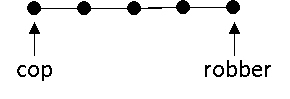
Once these values are assigned, the cop is put somewhere on the graph (whether she picks or is randomly placed somewhere).  The gambler is randomly placed by the computer at a vertex.  To make things simple let's just assume the graph looks like the one below.

If the gambler is placed at p3 then when it is his turn to move, there is a 25% chance he will move to v4 and a 15% chance he will move to v2.  The gambler is free to move anywhere, so he also has a 30% chance of landing on p1.  Since the gambler doesn't choose where he goes, the computer randomly chooses using these probability distributions as "weights".

Also keep in mind that when playing, the cop and gambler don't know where the other is positioned on the graph so in terms of the simulation there would be an "if condition" checking to see if the cop and gambler are on the same vertex.  If this part doesn't make sense, no worries, I am just using computer science jargon!

                                                   p1 = .3     p2 = .15      p3 = .3     p4 = .25

Thus, if we think about it in terms of a computer simulation we realize that it would be rather difficult to implement in reality.

On the bright side, it is pretty thoroughly proof-based so let’s get excited to do some proofs!!

https://media.giphy.com/media/dEdmW17JnZhiU/giphy.gif

Variations

• The cop knows the gamble (known gambler).
• In this case, the value of the game is exactly n regardless of the graph's structure or the cop's initial location.
• I will be focusing on this variation.
• The cop does not know the gamble (unknown gambler).

Before moving on to the proofs, just imagine that the gambler is your sweet grandmother because grandma’s love to gamble don’t they?  I know mine does!  Don’t tell her I put her on my blog...she’d get mad!

Cop                                        Gambler

By the way, it might be hard to see in the picture but those are lotteries, a bingo game, mega millions tickets, and my gram’s favorite slot game, Double Diamonds!  She loves them slots!!

Now, onto the proofs!

-- Cop & known gambler --

I apologize in advance for the layout of the proof (it is difficult to read).  Latex was putting everything on a new line so I instead used HTML code for the symbols.  Sorry it's not that easy to read!  I will be going over this proof in my presentation.

Lemma 5.1. The cop can capture the gambler in expected time less than or equal to n on Pn.

Proof
Strategy:  The cop moves from vi toward vn stopping when pi is large enough to allow it.

Suppose the cop is at vi.
Let mi = n - i + 1 be the total number of vertices ahead of the cop (including the one she is on now).
Let ci = pi + ... + pn be the sum of probabilities that are ahead of the cop (including the one she is on now).
Let Ti be the expected time from our current position until capture time.

Claim: Ti  ≤ mi /ci  for all i ϵ {1...n} proceeding by induction.
When mi = 1, i = n so the cop is at vn so cn = pn and therefore, Tn = 1/pn = mn / cn.
Suppose this holds for all mj for j > i and suppose the cop has arrived at vi.
If pi ≥ ci / mi we are done since Ti = 1/pi ≤ mi / ci.
Suppose that pi < ci / mi. With probability pi, the cop captures the gambler at vi (which takes 1) and with probability 1-pi, she moves on to vertex vi+1.
Now mi+1 = mi-1 < mi so the expected capture time from this new position is bounded by mi+1 / ci+1 = mi-1 / ci-pi. This yields the following inequality:
Ti ≤ 1 + (1 - pi)(mi-1 / ci-pi).
We have (for i > 1):
pi < ci / mi
→ ci(ci-1) < mipi(ci - 1)
→ ci(ci-mipi+mi-1+pi-pi) < mi(ci-pi)
→ ci / ci-pi (ci-pi+mi(1-pi)-(1-pi)) < mi
→ ci + (ci (1-pi) / ci-pi )(mi-1) < mi
→ 1 + (1-pi/ci-pi) (mi-1) < mi / ci
Therefore, Ti < mi / ci whenever pi < ci / mi as desired.

Intuitively:  Say we have a path with n vertices, and the cop starts on either end.  The cop travels from vertex to adjacent vertex and stops when the probability is large enough to allow it.  This proof is saying that there will always be a place where the cop can stop.  This will give us an expected capture time less than or equal to n.

If you have any questions about this proof, leave them in the comments section!

There are several other proofs that are involved in the game of Cop vs. Gambler that I will be going over on Thursday including:

Lemma 5.2. The cop can capture the gambler in expected time at most n on any tree of order n.

Lemma 5.3. The gambler can guarantee that the game takes at least n moves on average on any connected graph on n vertices.

Theorem 5.1. The value of the cop vs gambler game on any connected n-vertex graph is n.
→ consequently, since the cop has an upper bound of n and the gambler has a lower bound of n the        we end up having a game value equal to n.

From all of these proofs, we surprisingly find that the game value is n regardless of the graph we are using or the cop's initial starting position.

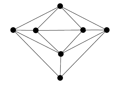
I will be doing some examples in my presentation that will apply these proofs and will use a graph that is similar to the one shown earlier.


-- Cop & unknown gambler --

I won’t be going in depth with this variation but I will explain the basics of it.

In this variant, the strategy is not known to the cop (private gamble) in which case the expected capture time will be different.  It turns out that the expected capture time is between n and 2n.  These are sort of the upper and lower bounds.

If you are particularly interested in this variant you can check out the proofs under the Cop & Unknown Gambler heading, here.

Conclusion

Cop vs. Gambler is more likely to appear in software design.  For example, imagine we have a program that prevents an attack (anti-incursion) and has to navigate a linked list of ports, trying to minimize the time to intercept an enemy packet as it arrives.  If the enemies’ port-choice is known then we get a version of the known gambler, otherwise we get a version of the unknown gambler.

Remember: Cop & Known Gambler à Our cop relied on knowing the gambler’s strategy (when the gamble was public).  This gave us an expected capture time of at most n.  The overall game value is n regardless of the graph or cop's initial position.

Cop vs. Gambler is a pursuit-evasion game that is a variant of the original Cop vs. Robber.  There is another variant that is similar to Cop vs. Gambler called Hunter vs. Mole that Jack will be talking about!

Sources

Natasha Komarov. “Cops Vs. Gambler.” August 23, 2013. Accessed March 1, 2017. https://arxiv.org/pdf/1308.4715.pdf.   
Natasha Komarov. “Capture Time in Variants of Cops & Robbers Games.” July 30, 2013. Accessed March 1, 2017. http://www.math.cmu.edu/~nkomarov/NKThesis.pdf.  

Cops and Robbers: Capture Time

Before I begin discussing the Capture Time of a game of Cops and Robbers, there a few important concepts of Natasha’s talk that should be kept in mind:

1. The neighborhood of a vertex, call it v, is a set containing all the vertices v is adjacent to. We will denote this N(v).
2. A vertex v dominates a vertex u if N(u) is a subset of N(v).
3. A corner is a vertex in a graph that a robber can lose from, or more mathematically stated, u is a corner if there is some vertex v in the graph such that v dominates u.
4. A graph is dismantlable if it has a sequence of corners which when removed result in the trivial graph (a single vertex).
5. A graph is cop-win if and only if it’s dismantlable.

Now that we have all this in mind, there is some new vocab to learn.

1. In a game of Cops and Robbers, the length of the game is how many rounds it takes to capture the robber.
2. When playing the game, the play is considered optimal if the cops capture the robber in the least amount of time, assuming the robber is trying to maximize the length of the game.
3. The length of the optimal game is what we call the capture time of G, denoted capt(G).

What this means in English is that if we have a game of Cops and Robbers, where the robber is avoiding capture for a long as possible, then the capture time of G is the minimum number of turns it takes the cops to capture him.

If you want some practice with this idea, feel free to try and work out the capture time for the graphs below, and leave your answer in the comments section. We’ll also work through these two examples in class, so don’t worry too much if this is still confusing. 

G1

G2

While it is relatively easy to determine the capture time of individual graphs, there are an infinite number of graphs, and it is impossible to compute the capture time of them all. For this reason, we need to characterize graphs to help us determine their capture time. The following proofs will help us to determine the upper bound on the capture time of certain types of graphs.

How can we determine Capture Time?

Theorem 1:

If G is a cop-win graph, then capt(G) ≤ n-1, where n is the number of vertices in G.

This proof is dense, but if you would like to read it, you can find it under the heading Theorem 1.2.3 here.

It is a rather logical argument though. Let’s think about the longest game it is possible to play on a cop-win graph. As an example, use the basic tree graph, with n vertices. If a cop starts at one end, and robber starts at the other, then the cop will always move closer to the robber while the robber will stay put. The longest time a game played this way will take is n-1 turns. This means n-1 is our upper bound for the capture time, so capt(G) ≤ n-1.

In an example with five vertices, the cop starts on the left side, while the robber starts on the right:

On each turn, the cop moves one closer to the robber.

So, the longest time this game can take is four turns, or the number of vertices minus one. We know the capture time must be smaller than or equal to this, since the capture time is the minimum number of turns it takes to win. And since there is no way to play this graph with five moves, our upper bound of n-1 (4 in this case) makes sense.

Improvement on the Upper Bound

We can do better than that though. It turns out the following is true:

If G is a cop-win graph of order n ≥ 5, then capt(G) ≤ n-3.

Proof by Induction:

Base Case: n=5

This holds true for n=5, because you can check all cop-win graphs of order 5 and see that it does.

Inductive Step:

Suppose the theorem holds true for graphs of order n≥5, and assume G has n+1 vertices.

Then G has a corner, u, and since by deleting that corner we get back to a graph with n vertices, the graph G is cop-win.

By the induction hypothesis, the cop can capture the robber in the graph G – u in at most n-3 rounds. So in G, if the robber is not on u, then the cop plays her winning strategy, and can win in n-3 rounds. If the robber is on u, then the cop will only be one vertex away and can win in (n+1)-3 moves.

For more information on this proof, see The Games of Cops and Robber on Graphs by Bonato and Nowakowski, page 36.

Further Improvement on the Upper Bound

It turns out we can do even better though. Some graphs have two separate corners, which when removed make another graph with two separate corners. If those two vertices can be removed, to make another graph with two separate corners, and so on until the graph has less than seven vertices, then the graph is called 2-dismantlable.

It turns out, if G is 2-dismantlable of order n, then capt(G) ≤ n/2.

This is another proof by induction, which I will leave as an exercise for the reader if they are so inclined. If not, you can find it in The Games of Cops and Robber on Graphs by Bonato and Nowakowski, page 216.

We'll do an example of this type of graph in class, because it's rather involved, but if you have any questions before than please leave them in the comments section!

More Improvement on the Upper Bound

The following characterization of graphs relates to the final example Natasha gave us on Thursday.

This graph belongs to a special group of graphs that we know the exact capture time of.

If a graph G is planar, cop-win with a unique corner and has n ≥ 7 vertices, then capt(G) = n-4.

So, what’s the capture time of the graph above? Three. In order for the cop to catch the robber, she needs at least three turns, assuming the robber plays optimally.

If you are interested in the proof for this theorem, see The Games of Cops and Robber on Graphs by Bonato and Nowakowski, page 217.

Capture Time with More Than One Cop

So far everything we’ve done has dealt with graphs that have a cop number of 1. What about graphs that need more cops? Research is still ongoing in this area, but the basic ideas of capture time apply the same way to graphs with more than one cop.

One example would be the 4-cycle graph from class, which needed two cops to make it cop-win.

What is the capture time of this graph? Leave your answer in the comments below.

Conclusion

The capture time of graph is important because it tells us how quickly the cops can catch the robber, even if the robber is trying to evade capture for as long as possible. There is no definite answer as to what the capture time of any given graph is, especially when you complicate it by adding more cops. Research is ongoing, and at the moment the best we can do to estimate the capture time of a graph is to use the bounds proven above. 

Citations:

Bonato, Anthony, and Richard J. Nowakowski. The Game of Cops and Robbers on Graphs. Providence, RI: American Mathematical Society, 2011. Print.

Bonato, A., P. Golovach, G. Hahn, and J. Kratochvi­l. "The Capture Time of a Graph."Discrete Mathematics 309.18 (2009): 5588-595. Web.

Clarke, Nancy E. Constrained Cops and Robbers. Diss. Dalhousie U, 2002. Ottawa: National Library of Canada, 2002. Print.

Green Hackenbush

Green Hackenbush

Green Hackenbush is an impartial combinatorial game. It is played on any configuration of green line segments connected to one another by their endpoints and to a "ground" line. I will call these green line segments "edges." From any position, exactly the same moves are legal for each of the two players. Green Hackenbush was invented by mathematician John Horton Conway who was born in 1937 and is still alive today!

How to Play:

• Two players take turns cutting edges on a connected rooted graph or a collection of connected rooted graphs.
• When a player cuts an edge, it disappears along with any edges that are no longer connected to the ground
• The player who cuts the last edge wins.
• We will assume there are finitely many edges on the board

A simple kind of green Hackenbush is a picture of green snakes, which consists of a chain of green edges with just one edge touching the ground. The ground is represented as the dotted line. We can bend the topmost edge into a loop so our snakes have heads because loops are essentially just another edge. The figure below illustrates this setup. The elements made of only one segment are perhaps better called blades of grass (or baby snakes?).

                        

Berlekamp, Elwyn R., Conway, John H., and Guy, Richard K.. Winning Ways for Your Mathematical Plays. Natick, US: A K Peters/CRC Press, 2002. ProQuest ebrary. Web. 19 February 2017. (p. 41)

We can see that in this game, any move will affect just one snake and will replace that snake by a shorter one. To find the position of this game, we will assign each snake a nimber. Because each snake is a single string of edges, the nimber of a snake is the number of edges. To find the position of the game, we nim-sum the nimbers together. So in the case of this game, we have 5 ⊕ 1 ⊕ 1 ⊕ 1 ⊕ 1 ⊕ 6 ⊕ 4 = 7. Just like in Nim, because the value is not zero, we are in a N-position.

Here’s a question for the comments below: How is the game-play of Green Hackenbush consisting of snakes and grass equivalent to Nim?

Here is some strategy for Green Hackenbush with green snakes (can you see the connection to Nim?):

•  A single snake can be won by the first player every time by chopping the bottom edge of the snake.
• Two snakes of equal size have a nim-sum of zero
• A game of two unequal snakes can be won by the first player every time if the first player can equalize them by reducing the larger one
• In a three snake game, the player who first equalizes two of the snakes or eliminates a snake is the loser. In the first case, the opponent can remove the third snake. In the second, the opponeent can equalize the two non-empty snakes.

But what if someone who suffers from Ophidiophobia wants to play Green Hackenbush? Or someone who wants to start with a more complex picture? We can use the Colon Principle to find the position of a game consisting of trees.

Colon Principle: When several stalks meet at a vertex we may replace those stalks by a single stalk of the value equal to their sum.

By using the Colon Principle, we can find the position of a tree/shrub consisting of two edges emanating from point a:

1 ⊕ 1 = 0

We can see that the nim-sum of the number of edges on each branch is zero. So, we can replace the edges coming from a with no edges. As we know, a nim-sum of zero means the game is in a P-position. This may be obvious, but the previous player (player 1) will win because player 2 will erase one edge, player 1 will erase the remaining edge, and player 2 will be left with no moves and thus be the loser.

Another example:

 

3 ⊕ 2 = 1

Because the nim-sum of the branches emanating from b is 1, we can replace them with a single edge emanating from b to find the position of this game.

Using the ideas discussed above and the Colon Principle, we can find the position of a game of Green Hackenbush with a more complex tree by simplifying at points where “branches” diverge through several steps.

Berlekamp, Elwyn R., Conway, John H., and Guy, Richard K.. Winning Ways for Your Mathematical Plays. Natick, US: A K Peters/CRC Press, 2002. ProQuest ebrary. Web. 19 February 2017. (p. 191)

From using the colon principle above, we can eliminate the two branches emanating from a, and we can replace the branches emanating from b with 1 edge (see above examples). Because there is a 2 edge branch and a 1 edge branch coming from c, we can nim-sum them (2 ⊕ 1 = 3), and replace them with 3 segments. Then, we nim-sum the number of edges in each branch emanating from d: 2 ⊕ 2 ⊕ 4 = 4. So, we replace the branches emanating from d with 4 edges. Therefore, this tree has a value of 5 because we are left with 5 edges in a single line/branch. Because this value is not zero, we know we are in an N-position. This is obvious because the next player can simply chop the “trunk” of the tree (the edge touching the ground), leaving the rest of the tree detached, thus eliminating the rest of the edges and winning the game.

We’ve mastered snakes and trees, but what if we want to play a game of Green Hackenbush that has a drawing with cycles? We can analyze that using the Fusion Principle. 

The Fusion Principle states that you can fuse all the nodes in any cycle of a Green Hackenbush picture without changing its value. You fuse two nodes of a picture by bringing them together into a single one. Any edge joining them gets bent into a loop. A loop at any node has the same effect as an edge.

A small example:

In the above example, we first fused c and a. The edge joining them is bent into the purple loop. The edge between b and a still exists but since c was fused with a, the edge between b and c is now between b and a. We then fused b and a. The edges between b and a are now loops, and we are left with three loops at a. These loops can be represented as edges. By using the Colon Principle, we nim-sum the three segments together: 1 ⊕ 1 ⊕ 1 = 1. So the original picture with the cycle between a, b, and c is an N-position.

We will discuss the proof of the Fusion Principle in class.

Now we can find the position of a game of Green Hackenbush consisting of a picture of anything made of edges, including this:

Here is an example of fusing a girl:

Berlekamp, Elwyn R., Conway, John H., and Guy, Richard K.. Winning Ways for Your Mathematical Plays. Natick, US: A K Peters/CRC Press, 2002. ProQuest ebrary. Web. 19 February 2017.  (p. 192)

We fused all of the nodes in the cycles and made the loops into edges. Can you find the value of the resulting tree by using the Colon Principle? 

More things to think about: What if there is a cycle that includes the ground? We will discuss this in class but feel free to leave your ideas in the comments.

Conclusion

There is a straightforward way to find the position of any game of Green Hackenbush. However, once you find the value of the position, it may not be so easy to determine what move to make to put the game into a P-position. This game may also be made partial by assigning two colors to the edges. In addition, Green Hackenbush Theory can be applied to several other games, including "Impartial Maundy Cake." 

Sources:

Berlekamp, Elwyn R., Conway, John H., and Guy, Richard K.. Winning Ways for Your Mathematical Plays. Natick, US: A K Peters/CRC Press, 2002. ProQuest ebrary. Web. 20 February 2017.

Esselstein, Rachel. Winning Strategies for Green Hackenbush. 2017. Web. 20 February 2017. http://merganser.math.gvsu.edu/david/reed05/projects/esselstein/msri/Esselstein/

Wikipedia. Hackenbush. February 2017. Web. 19 February 2017.